


Surface plasmon resonance, like all refractometric biosensors, suffers from environmental noise and needs very high measurement precision. To understand why, we need to know how the binding signal is acquired in this technique. We also need to know why it detects changes we are not interested in: noise.
Signal Processing- The Basics
Let’s begin by thinking of what we want to achieve with a biosensing technology such as SPR. Like most biosensors, the aim is to detect specific molecular interactions in real-time. But the bigger question we must ask first is: how can we measure only this specific molecular interaction and nothing else? In other words, how can we measure the signal without measuring the environmental noise buried in real space?
To develop such a sensing concept, we need a basic understanding of signal processing. This is not an easy task, mostly because the concepts used in signal processing quickly become abstract. To avoid confusion, we use an analogy for the molecular interactions we want to detect: a simple image from your smartphone camera. In the language of signal processing, a smartphone image and an array of molecular interactions is the same. So, what is an image, mathematically? It is just a combination of numbers, arranged in what we call a matrix (a table, of sorts). The numbers inside this matrix specify the intensity of light in the image at specific coordinates.
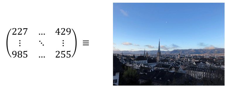
Often the biggest challenge in taking a photograph is to image what is in front of the camera, for example the faces of the people. In that respect it is very similar to detecting biosignals. The issue that both these processes face is also the same: noise. Noise is the range of signals we do not want to acquire. They interfere with the readout of the signal we do want, in our analogy the faces. It can come from environmental influences. If you take a picture facing the sun, the faces do not appear, because the sunlight overexposes your sensor. This issue stems from problems with data acquisition, e.g. the settings you use on your camera when taking a picture. One way to fix this is to account for environmental noise while the data is acquired. That is harder than it sounds. You do not always know where the noise will come from or how much it will interfere with the signal of interest. Usually, it only becomes evident once the data (in our example, still the image) is already acquired. However, this remains problematic, because not all environmental noise can be filtered out once the signal is obtained. Indeed, an overexposed photograph can be filtered to enhance certain contrasts, but filters cannot entirely remove the overexposed nature of the image. This is because every pixel in the image is immersed in environmental noise and these signals fully overlap: they can no longer be fully discriminated. For this reason, it is essential to exclude as much noise as possible before data acquisition. Filtering noise is the key to this; but how can it be achieved before signal acquisition? How is it different than using filters on a smartphone?
Filtering Signals
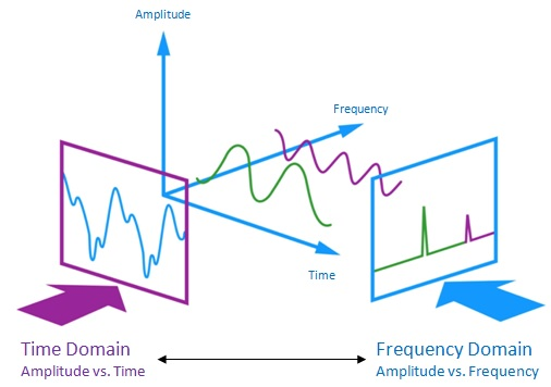
Filtering can be done in different ways, and more importantly, it can be done in different spaces: in real space, or in Fourier space. Real space describes space the way we are most familiar with it, the way we see it, in the typical three dimensions. Fourier space on the other hand isn’t a “space” the way we conceive it in our minds, but a mathematical analogy of this. It is used to convert images from the real space in terms of their frequency components. The tool that we use to perform this transformation is called the Fourier transform. What this looks like mathematically is a conversion of a complicated function (representing the raw signal or the raw image) into several simpler functions. Figure 1 depicts this concept. The raw signal shown in the time domain (in real space) can be separated into simpler components in the so-called frequency domain. When graphically representing these components in the frequency domain, we obtain a very different graph. The essential take-away: although the frequency domain graph looks very different, it represents the same original signal, just in a different manner.
Images in Fourier Space
Signals can be represented both in real space and in Fourier space; this applies to images as well! Below is an example of an image in real space (on the left) vs. image in Fourier space (on the right). In Fourier space, signals closest to the center are low-frequency signals, while high-frequency signals are found in the periphery.
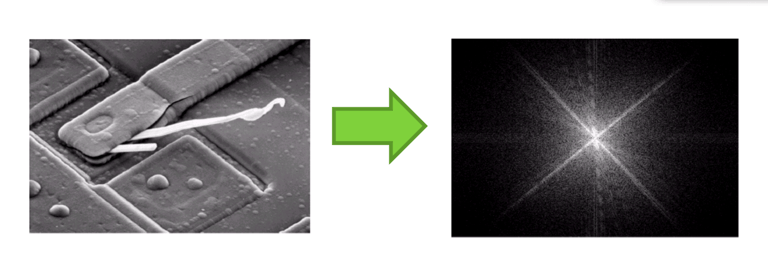
Although these images look vastly different, they represent the same information in different manners. In short: there is more than one way to see an image (and biosignals). Why is this important and why is it useful to represent biosignals and images in Fourier space instead of real space? It all comes back to the question at the beginning of this article. When we try to detect a specific signal or capture a specific image, how can we detect exactly what we want and nothing else? The answer to this is to perform the measurement in Fourier space instead of real space.
But why? Analyzing signals and images in real space is much more intuitive. Handling the data in this space once it is acquired is much harder. As mentioned, data acquisition is often faulty. We cannot always acquire our data in a way that excludes every unwanted signal. This is particularly difficult with biosignals, because we can not see environmental noise the way we do an image. This is why we must use filters before the data is acquired, unlike applying a filter to a taken image on our smartphones. Look at the signal acquired in the time domain in figure 1, for example. Filtering out the unwanted signal there is a tedious task. Just by looking at this function, how can we know what parts of it we want, and what parts we don’t want? Moreover, how can we remove those parts across the entire function? Likewise, for the image, how can we filter out the noise and keep the desired information? The truth is, unless we go through the process of trial and error, it is very difficult to do this in real space. However, when looking at the same information in Fourier space, things become much simpler. In the right image of figure 2, for instance, we see a bright spot in the middle that dims toward the edge. This means the image contains a lot of low-frequency signal (slow or long-ranged) and only little high-frequency signal (fast or short-ranged). Noisy signal happens to sit in the low-frequency range. Knowing this, we can simply filter out the signal in the center of the image and keep everything around it. Similarly, for the signal in figure 1, we can remove the peak at low frequency and keep the peak at high frequency. Once the filtering is done, the inverse Fourier transform converts the filtered data from Fourier space back into real space. The result is a “clean” signal that we can interpret.
Signals in Surface Plasmon Resonance
At this stage, it may be unclear how this relates to the surface plasmon resonance technology. The aim of SPR is to detect biosignals. The signals we want to detect with SPR are mixed with a much larger noise component that we are not interested in. We therefore face the problem described throughout this article: how to detect signal without noise. This matters for SPR in particular. Without a reliable way to solve it, the signal we want to detect is easily lost in a sea of noise. In practice, this is what makes SPR so challenging; it is extremely sensitive, but this sensitivity does not discriminate between desired signal and the noise. Indeed, SPR samples its data in real space. Every data point we sample contains noise and the weak signal is diluted over all. In order to get enough of the interesting signal, we need to sample many data points. This means that we acquire monumental amounts of noise.
Still confused? An analogy to put this into perspective.
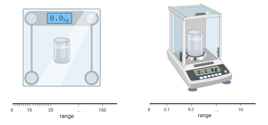
Imagine you are standing on a standard scale, one you would use to weigh yourself, with a shot glass containing a bit of water. In this analogy, you are the environmental noise. The water you pour into the glass is the signal, the change you want to detect. If a few drops of water are added to the shot glass, the scale you are standing on will most likely not detect the change. The increment is too small. To detect this change, that scale would need extremely high precision, down to the gram, while keeping a large weight range (0 to 100 kg). Weigh the shot glass alone on a new scale with a 0 to 10 g range, and the added weight of the water is detected. Thus, the new scale can detect the changes with higher accuracy. More importantly, the absolute precision required to detect the added water, 1 g in this example, is the same for both scales. In relative precision, however, the smaller scale has a large advantage. 1 g in a range of 10 g is a far less demanding precision than 1 g in a range of 100 kg. Surface plasmon resonance is like the big scale. It needs extremely high precision to detect the signals of interest, while also having to sample a very large range of signals.
In a Nutshell
How can we untangle these signals from each other across all the data points we sample? Could it be possible to avoid this problem and circumvent the noise acquisition completely? By sampling our data in Fourier space instead of real space, we achieve just that. Signal and noise are neatly separated. If we place our detector at the signal location, we acquire only the signal and do not even see the noise. This has a big advantage: our detector no longer requires extreme relative precision. We do not need a 100 kg scale with 1 g precision to measure a few drops of water added to a glass. In the same way, we do not need a signal detector that samples a large range with high precision. We can simply use a cheaper scale or signal detector with a much smaller range and much smaller relative precision. SPR measures signals the hard way; how can we design a biosensor that does this the smart way? Has such a biosensor ever been made? The next article answers this question.
References
http://play.fallows.ca/wp/radio/ham-radio/signal-analysis-morse-decoder/
biorender.com
Frutiger, Andreas, Christof Fattinger, and János Vörös. “Ultra-Stable Molecular Sensors by Sub-Micron Referencing and Why They Should Be Interrogated by Optical Diffraction—Part I. The Concept of a Spatial Affinity Lock-in Amplifier.” Sensors 21.2 (2021): 469.
Frutiger, Andreas, et al. “Ultra Stable Molecular Sensors by Submicron Referencing and Why They Should Be Interrogated by Optical Diffraction—Part II. Experimental Demonstration.” Sensors 21.1 (2021): 9.